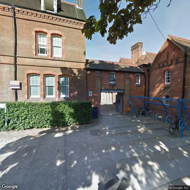
We wanted to put the Museum of English Rural Life
(The MERL) on Google Streetview to make us more accessible to those
with Autism Spectrum Disorder (ASD). For people with ASD it helps to
know what to expect at a place before they arrive, and Google Streetview
remains one of the most popular ways of scoping a place out. (Our offer
for people with ASD is forthcoming at the MERL.)
We thought it would be difficult to get on Streetview. What we didn’t realise is that:
pretty much anyone with the right equipment can put themselves on Google Streetview
it isn’t rocket science
So,
in this blog I’m going to tell you how we did it, in case you also want
to do it. If you want to skip straight to our Google Streetview tour, click here.
The background
In case you don’t know, Google Streetview
is attempting to capture every street in 360-degree photography. You
just drag the little yellow guy on Google Maps onto the street and have a
look.
The closest you could previously get in Streetview (hey, that’s my bike!)
Google Streetview also extends inside buildings, for which you used to have to hire a Trusted Pro to photograph your building. Google now allows anyone to do it themselves, kind of like what crowd-sourcing Panoramio used to be except for 360° photos.
The equipment
Google
will accept any photos taken with decent 360° cameras, and even accepts
photo spheres made with a normal smartphone camera if they’re good
enough. They have a very good page on how to publish for Google Streetview here.
These people are in exciting places but most of the 360 photos I’ve seen are of ducks on the canal and nail parlours
So,
technically you just need a smartphone, but the photo-spheres I’ve made
using just a normal camera almost always come out a bit glitchy. So I
suggest getting a real camera.
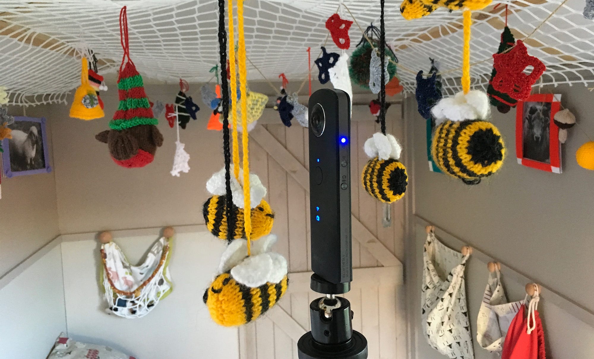
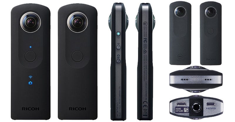
The
Theta-S takes images using two cameras on either side of its body, then
stitches them together for you. You just export the jpeg and upload it
onto something like Google Streetview or Facebook – sites which can
translate the file into an interactive photo-sphere.
Setting up the tour
So taking 360° photos is literally as easy as pressing a button, but planning the actual 360° tour? Not so much.
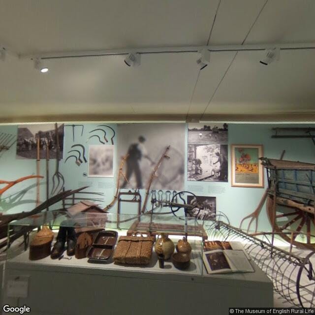
For
starters we didn’t want the photographer in the photo, so we mounted
the Theta S on a monopod and hid behind walls as we took the photo. This only failed once.
We
decided to capture the Museum while it was empty and shot on a Monday,
our closure day. Images of an empty museum, however, may give the wrong
impression of the museum to someone with ASD, as we usually have
visitors milling around. We plan to test this out with focus groups.
The ground floor had more than enough photos.
We
also wanted to be able to capture the whole museum, and planning our
tour was made easier by how our galleries are fairly one-way and linear.
Because
we only have our ground floor layer on Google Maps, though, we had to
miss out our first floor open store. We originally had both ground and
first floors published, but rapidly realised it was confusing people as
they kept switching randomly between floors in Streetview. We hope to
see whether getting our ground and first floor plans published on Google means we can then separate Streetview tours between them.
GO INSIDE WITH INDOOR MAPS WHENEVER GOOGLE CAN BE ARSED TO ACTUALLY UPLOAD YOUR SUBMISSION
Taking photos
Google
suggests taking photos a metre apart indoors, but we rarely kept to
this. On our first run we had a distance of something like five metres,
and then we went back to fill in some gaps.
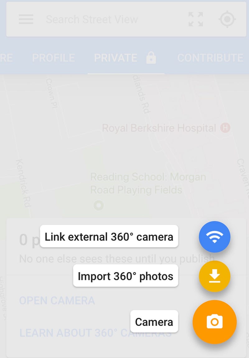
There’s
an option to connect the Google Streetview app to your 360° camera, but
we chose to take the photos and upload them separately (Import 360°
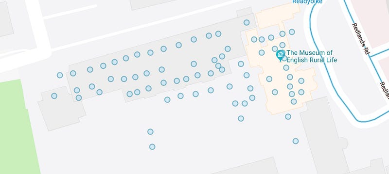
photos). I highly suggest taking all the photos you need, cut any
mistakes and then upload them all in one batch. If you have a museum the
size of the MERL you can do the whole museum in one go (76 photos), or
if you’re larger you could do it by gallery.
After
taking our photos we also realised some of them featured copyrighted
artworks. We opened these images in Photoshop, blurred out the artworks
and re-saved them – they still worked fine after editing, which was a
relief. The Google Streetview app also gives you the option of
automatically blurring faces.
Publishing
Once you have your photos collected you need to select all your photos and attach them to an address (i.e., your museum).
With
all the photos still selected, you then need to choose their precise
locations on Google Maps. This step is probably the most time-consuming.
As well as placing them in the exact spot you took them on your
floorplan, you also need to orient them to the compass so they’re
pointed in the right direction. This is very important for when you
connect your photos in a tour.
When
your photos are placed and oriented you can publish them to Google
Streetview. They usually show up fairly fast on the app and on desktop.
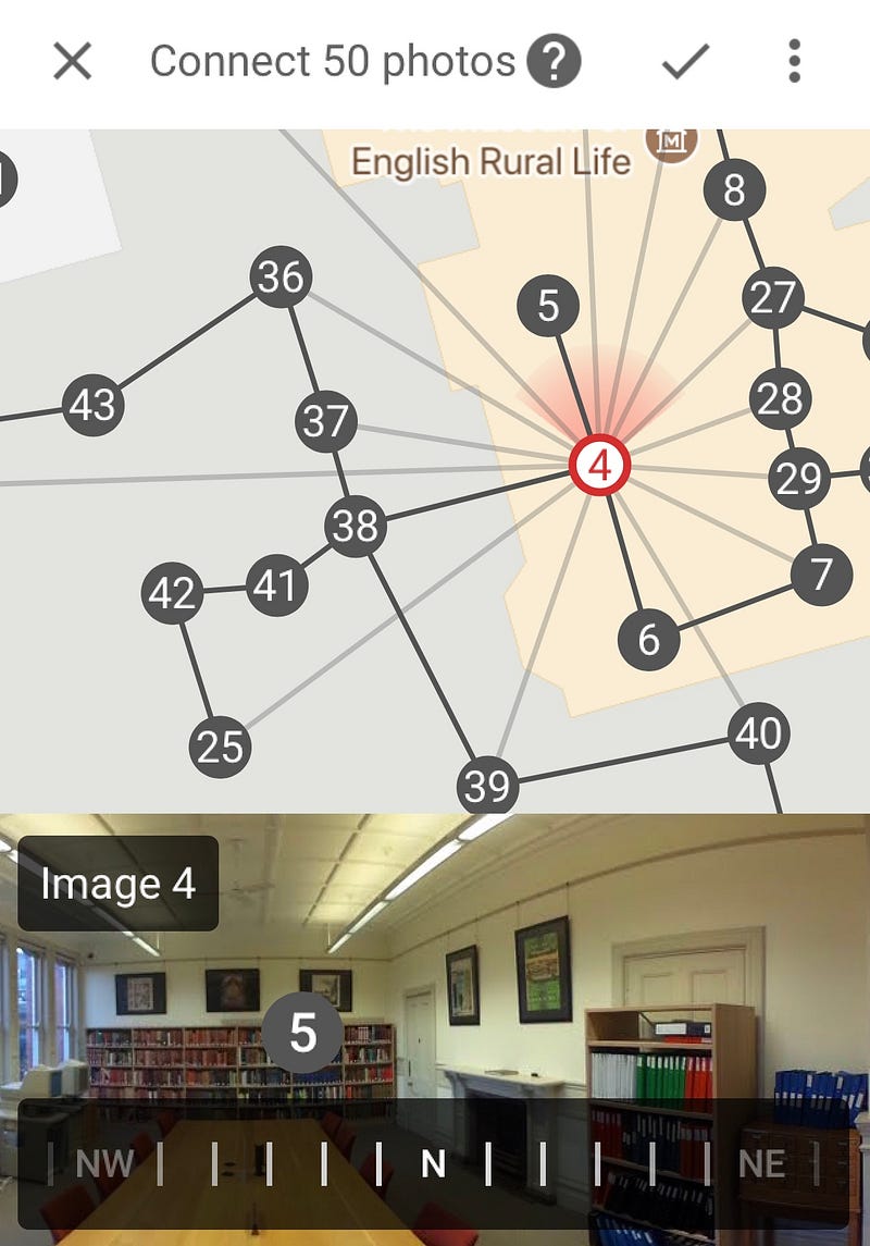
Connecting photos
The
beauty of Streetview is that you can place your photos in a sequential
tour. The option to link photos is only available after publication.
To do this I’d again suggest selecting all your photos at once, and then choosing the option to place and link.
You connect your photos by simply tapping the line between them, and you can link more than one picture to another.
That’s it.
It
updates instantly on the app, but it takes a couple of days before you
will be able to navigate through your photos on desktop using your
keyboard’s arrow keys or on your phone by tapping around.
The
aim of publishing our museum on Google Streetview is to prepare people
for what to expect at the Museum. It definitely accomplishes that.
We
considered photos and video, and have these options available too, but
nothing beats Streetview for giving the full picture. People already use
Google and Streetview, and it meant we could also embed the tour on our
website.
With
our planning, testing and re-runs the whole process probably took us
three full days of work. If you know what you need to capture, organise a
day for photography and dedicate the day to editing the photos then you
could easily get a museum the size of the MERL done in a day’s work.
A note on the Google Streetview app
I
don’t know whether it’s because I installed it on an iPad, but the
Google Streetview app is buggy as hell. It crashes, it is unresponsive
and often the map is completely obscured by cards. Prepare to be
frustrated, and work/save in batches to avoid losing your work.
Another
weird glitch which hasn’t been fixed yet is the option to transfer the
rights of your photos to the place where you took them. This is
primarily intended for Trusted Pros who are hired to make 360-degree
tours, and who then transfer the rights to the people who commissioned
the tour. It seemed strange that we could transfer rights to photos
taken using the MERL Google account to our same Google account tied to
the business. We did it anyway and all of our photos promptly
disappeared from Google Maps.
So, don’t do that until they’ve fixed it? But otherwise have fun.
The Historical Development of Machine Learning’s Core Structure
Why do we need Machine Learning?
Machine
learning is needed for tasks that are too complex for humans to code
directly. Some tasks are so complex that it is impractical, if not
impossible, for humans to work out all of the nuances and code for them
explicitly. So instead, we provide a large amount of data to a machine
learning algorithm and let the algorithm work it out by exploring that
data and searching for a model that will achieve what the programmers
have set it out to achieve.
Let’s look at these 2 examples:
It
is very hard to write programs that solve problems like recognizing a
3-dimensional object from a novel viewpoint in new lighting conditions
in a cluttered scene. We don’t know what program to write because we
don’t know how it’s done in our brain. Even if we had a good idea about
how to do it, the program might be horrendously complicated.
It is hard to write a program to compute the probability that a credit card transaction is fraudulent.
There may not be any rules that are both simple and reliable. We need
to combine a very large number of weak rules. Fraud is a moving target
but the program needs to keep changing.
Then comes the Machine Learning Approach:
Instead of writing a program by hand for each specific task, we collect
lots of examples that specify the correct output for a given input. A
machine learning algorithm then takes these examples and produces a
program that does the job. The program produced by the learning
algorithm may look very different from a typical hand-written program.
It may contain millions of numbers. If we do it right, the program works
for new cases as well as the ones we trained it on. If the data changes
the program can change too by training on the new data. You should note
that massive amounts of computation are now cheaper than paying someone
to write a task-specific program.
Given that, some examples of tasks best solved by machine learning include:
Recognizing patterns: Objects in real scenes, Facial identities or facial expressions, Spoken words
Recognizing
anomalies: Unusual sequences of credit card transactions, Unusual
patterns of sensor readings in a nuclear power plant
Prediction: Future stock prices or currency exchange rates, Which movies will a person like
What are Neural Networks?
Neural
networks are a class of models within the general machine learning
literature. So for example, if you took a Coursera course on machine
learning, neural networks will likely be covered. Neural networks are a
specific set of algorithms that has revolutionized the field of machine
learning. They are inspired by biological neural networks and the
current so called deep neural networks have proven to work quite very
well. Neural Networks are themselves general function approximations,
that is why they can be applied to literally almost any machine learning
problem where the problem is about learning a complex mapping from the
input to the output space.
Here are the 3 reasons to convince you to study neural computation:
To
understand how the brain actually works: It’s very big and very
complicated and made of stuff that dies when you poke it around. So we
need to use computer simulations.
To
understand a style of parallel computation inspired by neurons and
their adaptive connections: It’s a very different style from a
sequential computation.
To
solve practical problems by using novel learning algorithms inspired by
the brain: Learning algorithms can be very useful even if they are not
how the brain actually works.
After finishing the famous Andrew Ng’s Machine Learning Coursera course,
I started developing interest towards neural networks and deep
learning. Thus, I started looking at the best online resources to learn
about the topics and found Geoffrey Hinton’s Neural Networks for Machine Learning course.
If you are a deep learning practitioner or someone who want to get into
the deep learning/machine learning world, you should really take this
course. Geoffrey Hinton is without a doubt a godfather of the deep
learning world. And he actually provided something extraordinary in this
course. In this blog post, I want to share the 8 neural network architectures from the course that I believe any machine learning researchers should be familiar with to advance their work.
Generally, these architectures can be put into 3 specific categories:
1 — Feed-Forward Neural Networks
These
are the commonest type of neural network in practical applications. The
first layer is the input and the last layer is the output. If there is
more than one hidden layer, we call them “deep” neural networks. They
compute a series of transformations that change the similarities between
cases. The activities of the neurons in each layer are a non-linear
function of the activities in the layer below.
2 — Recurrent Networks
These
have directed cycles in their connection graph. That means you can
sometimes get back to where you started by following the arrows. They
can have complicated dynamics and this can make them very difficult to
train. They are more biologically realistic.
There
is a lot of interest at present in finding efficient ways of training
recurrent nets. Recurrent neural networks are a very natural way to
model sequential data. They are equivalent to very deep nets with one
hidden layer per time slice; except that they use the same weights at
every time slice and they get input at every time slice. They have the
ability to remember information in their hidden state for a long time
but is very hard to train them to use this potential.
3 — Symmetrically Connected Networks
These
are like recurrent networks, but the connections between units are
symmetrical (they have the same weight in both directions). Symmetric
networks are much easier to analyze than recurrent networks. They are
also more restricted in what they can do because they obey an energy
function. Symmetrically connected nets without hidden units are called
“Hopfield Nets.” Symmetrically connected network with hidden units are
called “Boltzmann machines.”
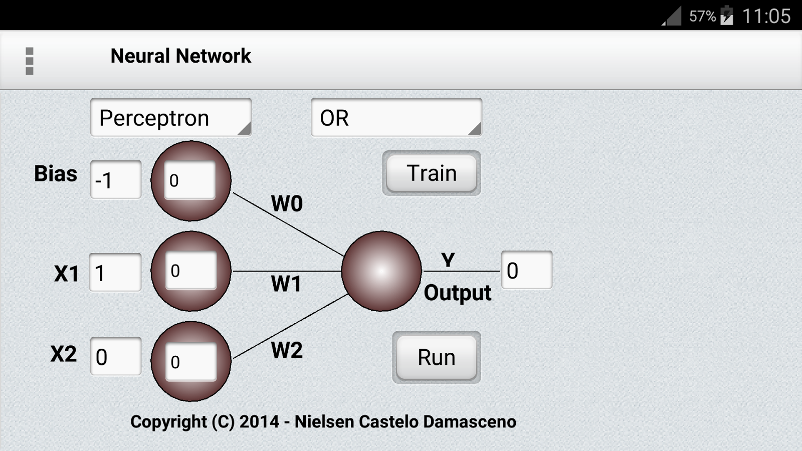
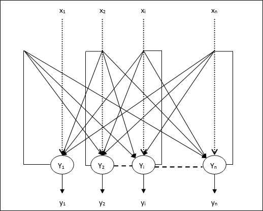
1 — Perceptrons
Considered the first generation of neural networks, perceptrons are simply computational models of a single neuron. They were popularized by Frank Rosenblatt
in the early 1960s. They appeared to have a very powerful learning
algorithm and lots of grand claims were made for what they could learn
to do. In 1969, Minsky and Papers published a book called “Perceptrons”
that analyzed what they could do and showed their limitations. Many
people thought these limitations applied to all neural network models.
However, the perceptron learning procedure is still widely used today
for tasks with enormous feature vectors that contain many millions of
features.
In
the standard paradigm for statistical pattern recognition, we first
convert the raw input vector into a vector of feature activations. We
then use hand-written programs based on common-sense to define the
features. Next, we learn how to weight each of the feature activations
to get a single scalar quantity. If this quantity is above some
threshold, we decide that the input vector is a positive example of the
target class.
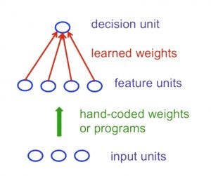
The
standard Perceptron architecture follows the feed-forward model,
meaning inputs are sent into the neuron, are processed, and result in an
output. In the diagram below, this means the network reads bottom-up:
input comes in from the bottom and output goes out from the top.
However,
Perceptrons do have limitations: If you are followed to choose the
features by hand and if you use enough features, you can do almost
anything. For binary input vectors, we can have a separate feature unit
for each of the exponentially many binary vectors and so we can make any
possible discrimination on binary input vectors. But once the
hand-coded features have been determined, there are very strong
limitations on what a perceptron can learn.
This
result is devastating for Perceptrons because the whole point of
pattern recognition is to recognize patterns despite transformations
like translation. Minsky and Papert’s “Group Invariance Theorem” says
that the part of a Perceptron that learns cannot learn to do this if the
transformations form a group. To deal with such transformations, a
Perceptron needs to use multiple feature units to recognize
transformations of informative sub-patterns. So the tricky part of
pattern recognition must be solved by the hand-coded feature detectors,
not the learning procedure.
Networks
without hidden units are very limited in the input-output mappings they
can learn to model. More layers of linear units do not help. It’s still
linear. Fixed output non-linearities are not enough. Thus, we need
multiple layers of adaptive, non-linear hidden units. But how we train
such nets? We need an efficient way of adapting all the weights, not
just the last layer. This is hard. Learning the weights going into
hidden units is equivalent to learning features. This is difficult
because nobody is telling us directly what the hidden units should do.
2 — Convolutional Neural Networks
Machine
Learning research has focused extensively on object detection problems
over the time. There are various things that make it hard to recognize
objects:
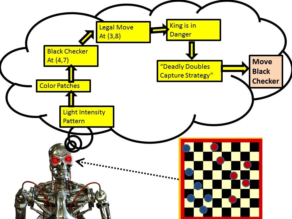
Segmentation:
Real scenes are cluttered with other objects. It’s hard to tell which
pieces go together as parts of the same object. Parts of an object can
be hidden behind other objects.
Lighting: The intensities of the pixels are determined as much by the lighting as by the objects.
Deformation: Objects can deform in a variety of non-affine ways. E.g., a handwritten too can have a large loop or just a cusp.
Affordances:
Object classes are often defined by how they are used. E.g., chairs are
things designed for sitting on so they have a wide variety of physical
shapes.
Viewpoint:
Changes in viewpoint cause changes in images that standard learning
methods cannot cope with. Information hops between input dimensions
(i.e. pixels)
Imagine
a medical database in which the age of a patient sometimes hopes to the
input dimension that normally codes for weight! To apply machine
learning we would first want to eliminate this dimension-hopping.
The
replicated feature approach is currently the dominant approach for
neural networks to solve object detection problem. It uses many
different copies of the same feature detector with different positions.
It could also replicate across scale and orientation, which is tricky
and expensive. Replication greatly reduces the number of free parameters
to be learned. It uses several different feature types, each with its
own map of replicated detectors. It also allows each patch of image to
be represented in several ways.
So what does replicating the feature detectors achieve?
Equivalent
activities: Replicated features do not make the neural activities
invariant to translation. The activities of are equivariant.
Invariant
knowledge: If a feature is useful in some locations during training,
detectors for that feature will be available in all locations during
testing.
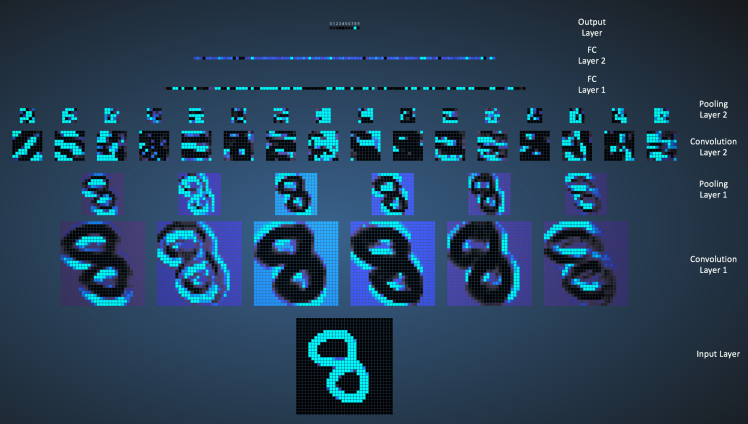
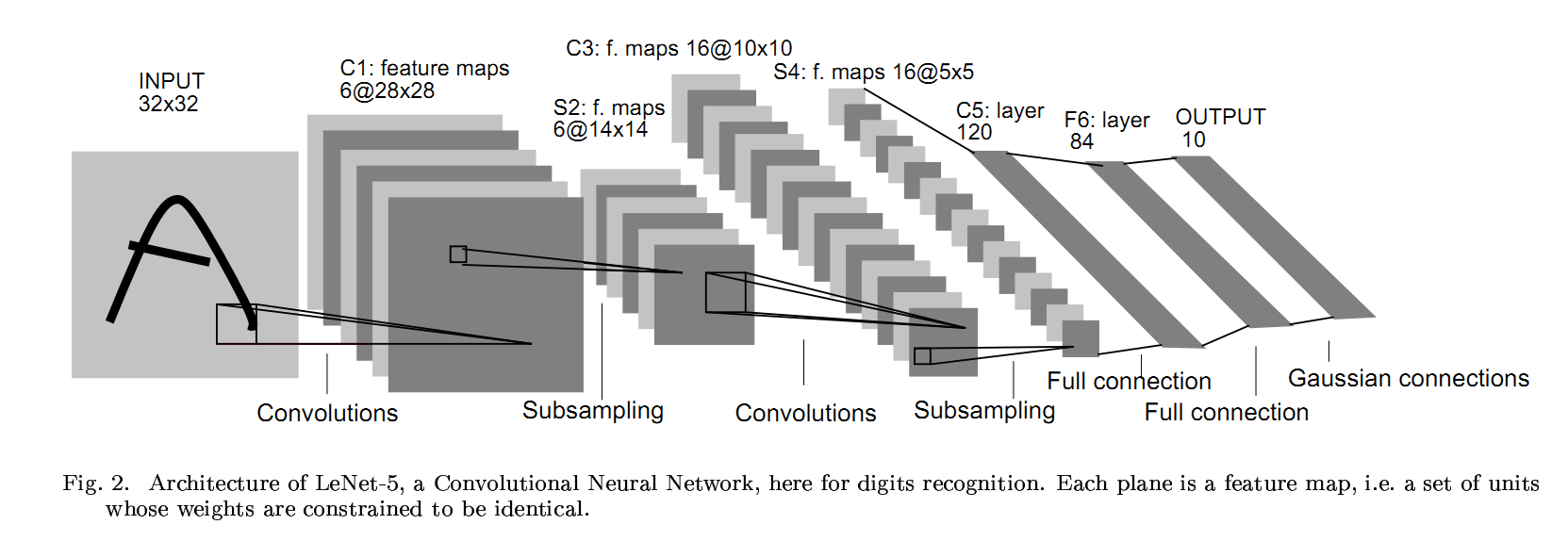
In 1998, Yann LeCun and his collaborators developed a really good recognizer for handwritten digits called LeNet.
It used back propagation in a feedforward net with many hidden layers,
many maps of replicated units in each layer, pooling of the outputs of
nearby replicated units, a wide net that can cope with several
characters at once even if they overlap, and a clever way of training a
complete system, not just a recognizer. Later it is formalized under the
name convolutional neural networks. Fun fact: This net was used for reading ~10% of the checks in North America.
Convolutional
Neural Networks can be used for all work related to object recognition
from hand-written digits to 3D objects. However, recognizing real
objects in color photographs downloaded from the web is much more
complicated than recognizing hand-written digits. There are hundred
times as many classes (1000 vs 10), hundred times as many pixels (256 x
256 color vs 28 x 28 gray), two-dimensional images of three-dimensional
scenes, cluttered scenes requiring segmentation, and multiple objects in
each image. Will the same type of convolutional neural network work?
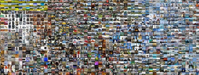
Then came the ILSVRC-2012 competition on ImageNet,
a dataset with approximately 1.2 million high-resolution training
images. Test images will be presented with no initial annotation (no
segmentation or labels) and algorithms will have to produce labelings
specifying what objects are present in the images. Some of the best
existing computer vision methods were tried on this dataset by leading
computer vision groups from Oxford, INRIA, XRCE… Typically, computer
vision systems use complicated multi-stage systems and the early stages
are typically hand-tuned by optimizing a few parameters.
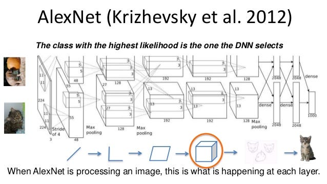
The winner of the competition, Alex Krizhevsky (NIPS 2012),
developed a very deep convolutional neural net of the type pioneered by
Yann LeCun. Its architecture includes 7 hidden layers not counting some
max-pooling layers. The early layers were convolutional, while the last
2 layers were globally connected. The activation functions were
rectified linear units in every hidden layer. These train much faster
and are more expressive than logistic units. In addition to that, it
also uses competitive normalization to suppress hidden activities when
nearby units have stronger activities. This helps with variations in
intensity.
There are a couple of technical tricks that significantly improve generalization for the neural net:
Training
on random 224 x 224 patches from the 256 x 256 images to get more data
and using left-right reflections of the images. At test time, combining
the opinions from 10 different patches: The four 224 x 224 corner
patches plus the central 224 x 224 patch plus the reflections of those 5
patches.
Using
“dropout” to regularize the weights in the globally connected layers
(which contain most of the parameters). Dropout means that half of the
hidden units in a layer are randomly removed for each training example.
This stops hidden units from relying too much on other hidden units.
In
terms of hardware requirement, Alex uses a very efficient
implementation of convolutional nets on 2 Nvidia GTX 580 GPUs (over 1000
fast little cores). The GPUs are very good for matrix-matrix multiplies
and also have very high bandwidth to memory. This allows him to train
the network in a week and makes it quick to combine results from 10
patches at test time. We can spread a network over many cores if we can
communicate the states fast enough. As cores get cheaper and datasets
get bigger, big neural nets will improve faster than old-fashioned
computer vision systems.
3 — Recurrent Neural Network
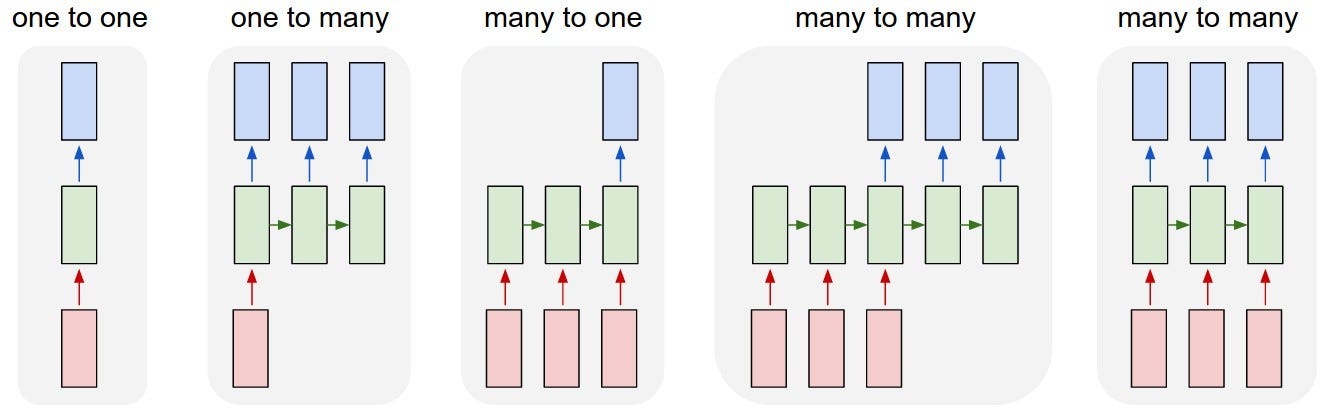
To
understand RNNs, we need to have a brief overview of sequence modeling.
When applying machine learning to sequences, we often want to turn an
input sequence into an output sequence that lives in a different domain;
for example, turn a sequence of sound pressures into a sequence of word
identities. When there is no separate target sequence, we can get a
teaching signal by trying to predict the next term in the input
sequence. The target output sequence is the input sequence with an
advance of 1 step. This seems much more natural than trying to predict
one pixel in an image from the other pixels, or one patch of an image
from the rest of the image. Predicting the next term in a sequence blurs
the distinction between supervised and unsupervised learning. It uses
methods designed for supervised learning, but it doesn’t require a
separate teaching signal.
Memoryless models
are the standard approach to this task. In particular, autoregressive
models can predict the next term in a sequence from a fixed number of
previous terms using “delay taps; and feed-forward neural nets are
generalized autoregressive models that use one or more layers of
non-linear hidden units. However, if we give our generative model some
hidden state, and if we give this hidden state its own internal
dynamics, we get a much more interesting kind of model: It can store
information in its hidden state for a long time. If the dynamics are
noisy and the way they generate outputs from their hidden state is
noisy, we can never know its exact hidden state. The best we can do is
to infer a probability distribution over the space of hidden state
vectors. This inference is only tractable for 2 types of hidden state
model.
Recurrent Neural Networks are
very powerful, because they combine 2 properties: 1) distributed hidden
state that allows them to store a lot of information about the past
efficiently, and 2) non-linear dynamics that allow them to update their
hidden state in complicated ways. With enough neurons and time, RNNs can
compute anything that can be computed by your computer. So what kinds
of behavior can RNNs exhibit? They can oscillate, they can settle to
point attractors, they can behave chaotically. And they could
potentially learn to implement lots of small programs that each capture a
nugget of knowledge and run in parallel, interacting to produce very
complicated effects.
However,
the computational power of RNNs makes them very hard to train. It is
quite difficult to train a RNN because of the exploding or vanishing
gradients problem. As we backpropagate through many layers, what happens
to the magnitude of the gradients? If the weights are small, the
gradients shrink exponentially. If the weights are big, the gradients
grow exponentially. Typical feed-forward neural nets can cope with these
exponential effects because they only have a few hidden layers. On the
other hand, in a RNN trained on long sequences, the gradients can easily
explode or vanish. Even with good initial weights, it’s very hard to
detect that the current target output depends on an input from many
time-steps ago, so RNNs have difficulty dealing with long-range
dependencies.
There are essentially 4 effective ways to learn a RNN:
Long Short Term Memory: Make the RNN out of little modules that are designed to remember values for a long time.
Hessian Free Optimization:
Deal with the vanishing gradients problem by using a fancy optimizer
that can detect directions with a tiny gradient but even smaller
curvature.
Echo State Networks:
Initialize the input -> hidden and hidden -> hidden and output
-> hidden connections very carefully so that the hidden state has a
huge reservoir of weakly coupled oscillators which can be selectively
driven by the input.
Good initialization with momentum: Initialize like in Echo State Networks, but then learn all of the connections using momentum.
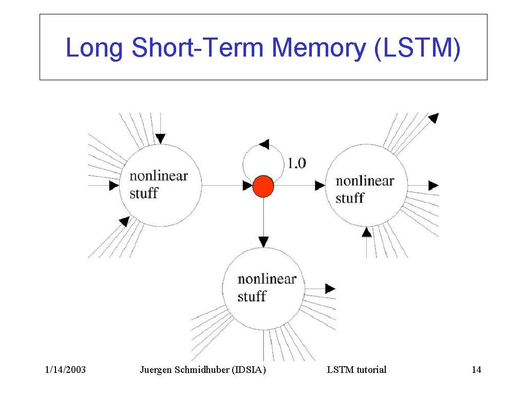
4 — Long/Short Term Memory Network
Hochreiter & Schmidhuber (1997) solved the problem of getting a RNN to remember things for a long time (like hundreds of time steps) by building what known as long-short term memory network. They
designed a memory cell using logistic and linear units with
multiplicative interactions. Information gets into the cell whenever its
“write” gate is on. The information stays in the cell so long as its
“keep” gate is on. Information can be read from the cell by turning on
its “read” gate.
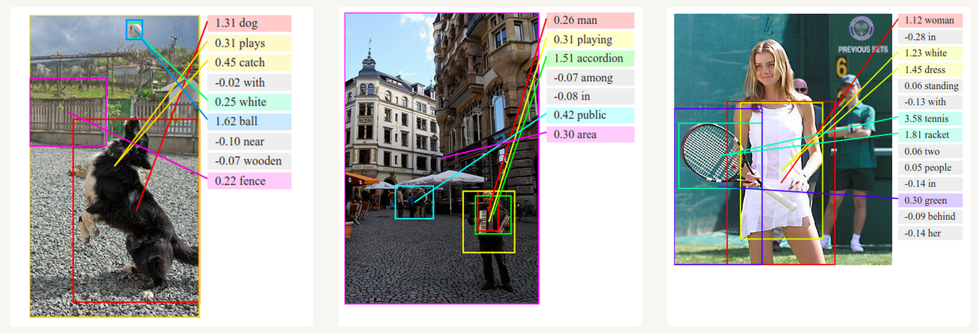
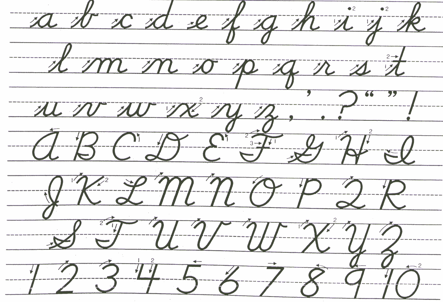
Reading
cursive handwriting is a natural task for an RNN. The input is a
sequence of (x, y, p) coordinates of the tip of the pen, where p
indicates whether the pen is up or down. The output is a sequence of
characters. Graves & Schmidhuber (2009)
showed that RNNs with LSTM are currently the best systems for reading
cursive writing. In brief, they used a sequence of small images as input
rather than pen coordinates.
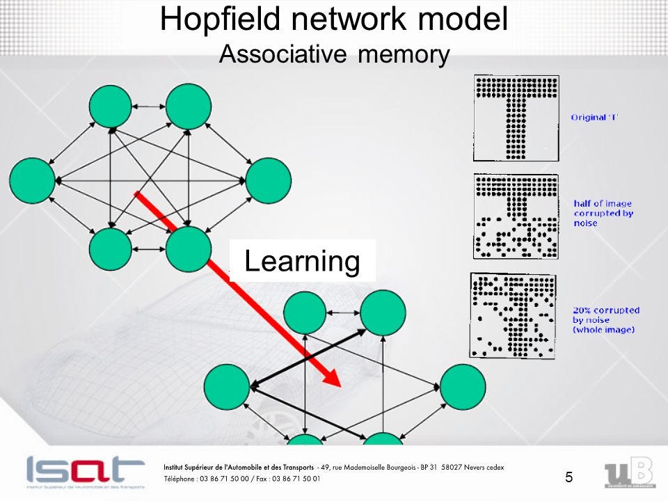
5 — Hopfield Networks
Recurrent
networks of non-linear units are generally very hard to analyze. They
can behave in many different ways: settle to a stable state, oscillate,
or follow chaotic trajectories that cannot be predicted far into the
future. A Hopfield net is composed of binary threshold units with recurrent connections between them. In 1982, John Hopfield
realized that if the connections are symmetric, there is a global
energy function. Each binary “configuration” of the whole network has an
energy; while the binary threshold decision rule causes the network to
settle for a minimum of this energy function. A neat way to make use of
this type of computation is to use memories as energy minima for the
neural net. Using energy minima to represent memories gives a
content-addressable memory. An item can be accessed by just knowing part
of its content. It is robust against hardware damage.
Each
time we memorize a configuration, we hope to create a new energy
minimum. But what if two nearby minima at an intermediate location? This
limits the capacity of a Hopfield net. So how do we increase the
capacity of a Hopfield net? Physicists love the idea that the math they
already know might explain how the brain works. Many papers were
published in physics journals about Hopfield nets and their storage
capacity. Eventually, Elizabeth Gardnerfigured
out that there was a much better storage rule that uses the full
capacity of the weights. Instead of trying to store vectors in one shot,
she cycled through the training set many times and used the perceptron
convergence procedure to train each unit to have the correct state given
the states of all the other units in that vector. Statisticians call
this technique “pseudo-likelihood.”
There
is another computational role for Hopfield nets. Instead of using the
net to store memories, we use it to construct interpretations of sensory
input. The input is represented by the visible units, the
interpretation is represented by the states of the hidden units, and the
badness of the interpretation is represented by the energy.
6 — Boltzmann Machine Network
A Boltzmann machine
is a type of stochastic recurrent neural network. It can be seen as the
stochastic, generative counterpart of Hopfield nets. It was one of the
first neural networks capable of learning internal representations and
is able to represent and solve difficult combinatoric problems.
The
goal of learning for Boltzmann machine learning algorithm is to
maximize the product of the probabilities that the Boltzmann machine
assigns to the binary vectors in the training set. This is equivalent to
maximizing the sum of the log probabilities that the Boltzmann machine
assigns to the training vectors. It is also equivalent to maximizing the
probability that we would obtain exactly the N training cases if we did
the following: 1) Let the network settle to its stationary distribution
N different time with no external input; and 2) Sample the visible
vector once each time.
For
the positive phase, first initialize the hidden probabilities at 0.5,
then clamp a data vector on the visible units, then update all the
hidden units in parallel until convergence using mean field updates.
After the net has converged, record PiPj for every connected pair of
units and average this over all data in the mini-batch.
For
the negative phase: first keep a set of “fantasy particles.” Each
particle has a value that is a global configuration. Then sequentially
update all the units in each fantasy particle a few times. For every
connected pair of units, average SiSj over all the fantasy particles.
In
a general Boltzmann machine, the stochastic updates of units need to be
sequential. There is a special architecture that allows alternating
parallel updates which are much more efficient (no connections within a
layer, no skip-layer connections). This mini-batch procedure makes the
updates of the Boltzmann machine more parallel. This is called a Deep
Boltzmann Machine (DBM), a general Boltzmann machine with a lot of
missing connections.
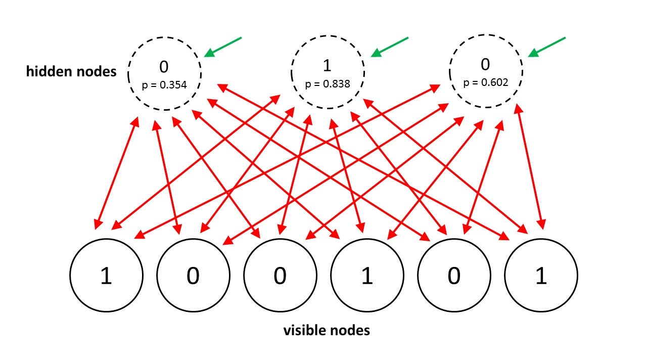
In 2014, Salakhutdinov and Hinton came up with another update for their model, calling it Restricted Boltzmann Machines.
They restrict the connectivity to make inference and learning easier
(only one layer of hidden units and no connections between hidden
units). In an RBM it only takes one step to reach thermal equilibrium
when the visible units are clamped.
Another efficient mini-batch learning procedure for RBM goes like this:
For
the positive phase, first clamp a data vector on the visible units.
Then compute the exact value of <ViHj> for all pairs of a visible
and a hidden unit. For every connected pair of units, average
<ViHj> over all data in the mini-batch.
For
the negative phase, also keep a set of “fantasy particles.” Then update
each fantasy particle a few times using alternating parallel updates.
For every connected pair of units, average ViHj over all the fantasy
particles.
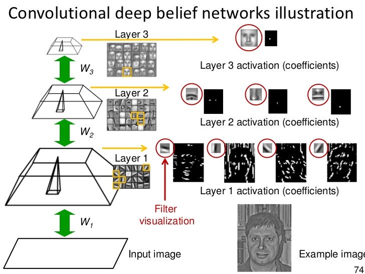
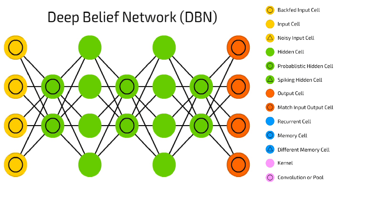
7 — Deep Belief Network
Back-propagation
is considered the standard method in artificial neural networks to
calculate the error contribution of each neuron after a batch of data is
processed. However, there are some major problems using
back-propagation. Firstly, it requires labeled training data; while
almost all data is unlabeled. Secondly, the learning time does not scale
well, which means it is very slow in networks with multiple hidden
layers. Thirdly, it can get stuck in poor local optima, so for deep nets
they are far from optimal.
To
overcome the limitations of back-propagation, researchers have
considered using unsupervised learning approaches. This helps keep the
efficiency and simplicity of using a gradient method for adjusting the
weights, but also use it for modeling the structure of the sensory
input. In particular, they adjust the weights to maximize the
probability that a generative model would have generated the sensory
input. The question is what kind of generative model should we learn?
Can it be an energy-based model like a Boltzmann machine? Or a causal
model made of idealized neurons? Or a hybrid of the two?
A belief net
is a directed acyclic graph composed of stochastic variables. Using
belief net, we get to observe some of the variables and we would like to
solve 2 problems: 1) The inference problem: Infer the states of the
unobserved variables, and 2) The learning problem: Adjust the
interactions between variables to make the network more likely to
generate the training data.
Early
graphical models used experts to define the graph structure and the
conditional probabilities. By then, the graphs were sparsely connected;
so researchers initially focused on doing correct inference, not on
learning. For neural nets, learning was central and hand-writing the
knowledge was not cool, because knowledge came from learning the
training data. Neural networks did not aim for interpretability or
sparse connectivity to make inference easy. Nevertheless, there are
neural network versions of belief nets.
There are two types of generative neural network composed of stochastic binary neurons: 1) Energy-based, in which we connect binary stochastic neurons using symmetric connections to get a Boltzmann Machine; and 2) Causal,
in which we connect binary stochastic neurons in a directed acyclic
graph to get a Sigmoid Belief Net. The descriptions of these two types
go beyond the scope of this article.
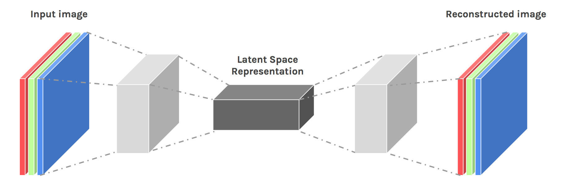
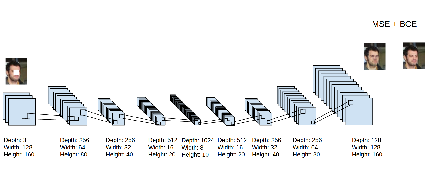
8 — Deep Auto-encoders
Finally, let’s discuss deep auto-encoders. They
always looked like a really nice way to do non-linear dimensionality
reduction because of a few reasons: They provide flexible mappings both
ways. The learning time is linear (or better) in the number of training
cases. And the final encoding model is fairly compact and fast. However,
it turned out to be very difficult to optimize deep auto encoders using
back propagation. With small initial weights, the back propagated
gradient dies. We now have a much better ways to optimize them; either
use unsupervised layer-by-layer pre-training or just initialize the
weights carefully as in Echo-State Nets.
For pre-training task, there are actually 3 different types of shallow auto-encoders:
RBM’s as auto-encoders:
When we train an RBM with one-step contrastive divergence, it tries to
make the reconstructions look like data. It’s like an auto encoder, but
it’s strongly regularized by using binary activities in the hidden
layer. When trained with maximum likelihood, RBMs are not like auto
encoders. We can replace the stack of RBM’s used for pre-training by a
stack of shallow auto encoders; however pre-training is not as effective
(for subsequent discrimination) if the shallow auto encoders are
regularized by penalizing the squared weights.
Denoising auto encoders:
These add noise to the input vector by setting many of its components
to 0 (like dropout, but for inputs). They are still required to
reconstructing these components so they must extract features that
capture correlations between inputs. Pre-training is very effective if
we use a stack of denoting auto encoders. It’s as good as or better than
pre-training with RBMs. It’s also simpler to evaluate the pre-training
because we can easily compute the value of the objective function. It
lacks the nice variational bound we get with RBMs, but this is only of
theoretical interest.
Contractive auto encoders:
Another way to regularize an auto encoder is to try to make the
activities of the hidden units as insensitive as possible to the inputs;
but they cannot just ignore the inputs because they must reconstruct
them. We achieve this by penalizing the squared gradient of each hidden
activity with respect to the inputs. Contractive auto encoders work very
well for pre-training. The codes tend to have the property that only a
small subset of the hidden units are sensitive to changes in the input.
In
brief, there are now many different ways to do layer-by-layer
pre-training of features. For datasets that do not have huge numbers of
labeled cases, pre-training helps subsequent discriminative learning.
For very large, labeled datasets, initializing the weights used in
supervised learning by using unsupervised pre-training is not necessary,
even for deep nets. Pre-training was the first good way to initialize
the weights for deep nets, but now there are other ways. But if we make
the nets much larger, we will need pre-training again!
Last Takeaway
Neural
networks are one of the most beautiful programming paradigms ever
invented. In the conventional approach to programming, we tell the
computer what to do, breaking big problems up into many small, precisely
defined tasks that the computer can easily perform. By contrast, in a
neural network we don’t tell the computer how to solve our problem.
Instead, it learns from observational data, figuring out its own
solution to the problem at hand.
Today,
deep neural networks and deep learning achieve outstanding performance
on many important problems in computer vision, speech recognition, and
natural language processing. They’re being deployed on a large scale by
companies such as Google, Microsoft, and Facebook.
I
hope that this post helps you learn the core concepts of neural
networks, including modern techniques for deep learning. You can get all
the lecture slides, research papers and programming assignments I have
done for Dr. Hinton’s Coursera course from my GitHub repo here. Good luck studying!
Face
recognition is the latest trend when it comes to user authentication.
Apple recently launched their new iPhone X which uses Face ID to authenticate users. OnePlus 5 is getting the Face Unlock feature from theOnePlus 5T soon. And Baidu is using face recognition instead of ID cards to allow their employees to enter their offices.
These applications may seem like magic to a lot of people. But in this
article we aim to demystify the subject by teaching you how to make your
own simplified version of a face recognition system in Python.
Before
we get into the details of the implementation I want to discuss the
details of FaceNet. Which is the network we will be using in our system.
FaceNet
FaceNet is a neural network that learns a mapping from face images to a compact Euclidean space
where distances correspond to a measure of face similarity. That is to
say, the more similar two face images are the lesser the distance
between them.
Triplet Loss
FaceNet
uses a distinct loss method called Triplet Loss to calculate loss.
Triplet Loss minimises the distance between an anchor and a positive,
images that contain same identity, and maximises the distance between
the anchor and a negative, images that contain different identities.
Figure 1: The Triplet Loss equation
f(a) refers to the output encoding of the anchor
f(p) refers to the output encoding of the positive
f(n) refers to the output encoding of the negative
alpha is a constant used to make sure that the network does not try to optimise towards f(a) - f(p) = f(a) - f(n) = 0.
[…]+ is equal to max(0, sum)
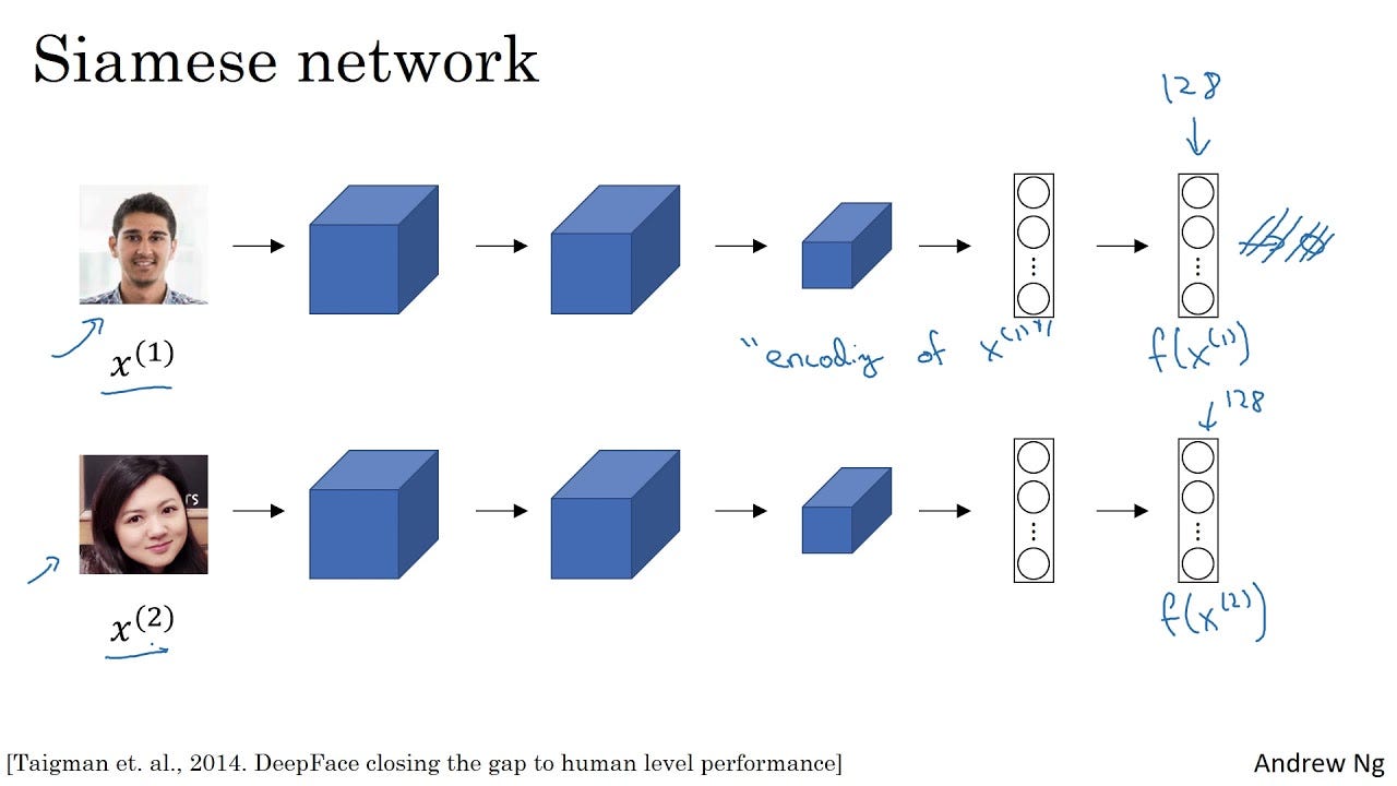
Siamese Networks
Figure
2: An example of a Siamese network that uses images of faces as input
and outputs a 128 number encoding of the image. Source: Coursera
FaceNet
is a Siamese Network. A Siamese Network is a type of neural network
architecture that learns how to differentiate between two inputs. This
allows them to learn which images are similar and which are not. These
images could be contain faces.
Siamese
networks consist of two identical neural networks, each with the same
exact weights. First, each network take one of the two input images as
input. Then, the outputs of the last layers of each network are sent to a
function that determines whether the images contain the same identity.
In FaceNet, this is done by calculating the distance between the two outputs.
Implementation
Now that we have clarified the theory, we can jump straight into the implementation.
In our implementation we’re going to be using Keras and Tensorflow. Additionally, we’re using two utility files that we got from deeplearning.ai’s repo to abstract all interactions with the FaceNet network.:
fr_utils.py contains functions to feed images to the network and getting the encoding of images
inception_blocks_v2.py contains functions to prepare and compile the FaceNet network
Compiling the FaceNet network
The first thing we have to do is compile the FaceNet network so that we can use it for our face recognition system.
import os
import glob
import numpy as np
import cv2
import tensorflow as tf
from fr_utils import *
from inception_blocks_v2 import *
from keras import backend as K
FRmodel.compile(optimizer = 'adam', loss = triplet_loss, metrics = ['accuracy'])
load_weights_from_FaceNet(FRmodel)
We’ll
start by initialising our network with an input shape of (3, 96, 96).
That means that the Red-Green-Blue (RGB) channels are the first
dimension of the image volume fed to the network. And that all images
that are fed to the network must be 96x96 pixel images.
Next
we’ll define the Triplet Loss function. The function in the code
snippet above follows the definition of the Triplet Loss equation that
we defined in the previous section.
If
you are unfamiliar with any of the Tensorflow functions used to perform
the calculation, I’d recommend reading the documentation (for which I
have added links to for each function) as it will improve your
understanding of the code. But comparing the function to the equation in
Figure 1 should be enough.
Once we have our loss function, we can compile our face recognition model using Keras. And we’ll use the Adam optimizer to minimise the loss calculated by the Triplet Loss function.
Preparing a Database
Now
that we have compiled FaceNet, we are going to prepare a database of
individuals we want our system to recognise. We are going to use all the
images contained in our imagesdirectory for our database of individuals.
NOTE:
We are only going to use one image of each individual in our
implementation. The reason is that the FaceNet network is powerful
enough to only need one image of an individual to recognise them!
def prepare_database():
    database = {}
    for file in glob.glob("images/*"):
        identity = os.path.splitext(os.path.basename(file))[0]
        database[identity] = img_path_to_encoding(file, FRmodel)
return database
For each image, we will convert the image data to an encoding of 128 float numbers. We do this by calling the function img_path_to_encoding.
The function takes in a path to an image and feeds the image to our
face recognition network. Then, it returns the output from the network,
which happens to be the encoding of the image.
Once we have added the encoding for each image to our database, our system can finally start recognising individuals!
Recognising a Face
As
discussed in the Background section, FaceNet is trained to minimise the
distance between images of the same individual and maximise the
distance between images of different individuals. Our implementation
uses this information to determine which individual the new image fed to
our system is most likely to be.
def who_is_it(image, database, model):
    encoding = img_to_encoding(image, model)

    min_dist = 100
    identity = None

    # Loop over the database dictionary's names and encodings.
    for (name, db_enc) in database.items():
        dist = np.linalg.norm(db_enc - encoding)
print('distance for %s is %s' %(name, dist))
        if dist < min_dist:
            min_dist = dist
            identity = name

    if min_dist > 0.52:
        return None
    else:
        return identity
The function above feeds the new image into a utility function called img_to_encoding.
The function processes an image using FaceNet and returns the encoding
of the image. Now that we have the encoding we can find the individual
that the image most likely belongs to.
To
find the individual, we go through our database and calculate the
distance between our new image and each individual in the database. The
individual with the lowest distance to the new image is then chosen as
the most likely candidate.
Finally,
we must determine whether the candidate image and the new image contain
the same person or not. Since by the end of our loop we have only
determined the most likely individual. This is where the following code
snippet comes into play.
if min_dist > 0.52:
    return None
else:
    return identity
If the distance is above 0.52, then we determine that the individual in the new image does not exist in our database.
But, if the distance is equal to or below 0.52, then we determine they are the same individual!
Now
the tricky part here is that the value 0.52 was achieved through
trial-and-error on my behalf for my specific dataset. The best value
might be much lower or slightly higher and it will depend on your
implementation and data. I recommend trying out different values and see
what fits your system best!
Building a System using Face Recognition
Now
that we know the details on how we recognise a person using a face
recognition algorithm, we can start having some fun with it.
In
the Github repository I linked to at the beginning of this article is a
demo that uses a laptop’s webcam to feed video frames to our face
recognition algorithm. Once the algorithm recognises an individual in
the frame, the demo plays an audio message that welcomes the user using
the name of their image in the database. Figure 3 shows an example of
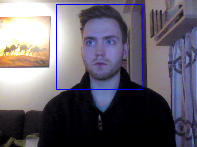
the demo in action.
Figure
3: An image captured at the exact moment when the network recognised
the individual in the image. The name of the image in the database was
“skuli.jpg” so the audio message played was “Welcome skuli, have a
nice day!”
Conclusion
By
now you should be familiar with how face recognition systems work and
how to make your own simplified face recognition system using a
pre-trained version of the FaceNet network in python!
If
you want to play around with the demonstration in the Github repository
and add images of people you know then go ahead and fork the
repository.
Have some fun with the demonstration and impress all your friends with your awesome knowledge of face recognition!
Hardik Gandhi is Master of Computer science,blogger,developer,SEO provider,Motivator and writes a Gujarati and Programming books and Advicer of career and all type of guidance.